
Part 2: Steel thread first: a practical data pipeline architecture
Learn how to build a sound data pipeline architecture, from the ground up, using an iterative approach that ships fast and scales.
In this second article on data pipelines I’ll show you how to build a foundational data pipeline architecture that stays true to requirements. At the same time, we’ll keep the architecture sound and simple; something we can scale, but also something we can build quickly. This aligns with the idea of launching a steel thread — rapidly delivering an architecturally complete system.
In the previous article I introduced data pipelines, highlighting their ubiquity and a few of the challenges you’ll face architecting a good data pipeline. Here’s a quick recap of those requirements:
Moving data efficiently. Pipelines are all about making sure the right data gets to the right place at the right time, in the right format. For many applications, like air traffic control or the stock market, timing is everything. The architecture has to scale, meeting demand without degrading — often with life-saving implications.
Data integrity. This is about ensuring the source data is what we think it is — incorruptible, unchanged as it moves through the pipeline. We have to make sure there’s no data loss, no translation errors, no dropped information. Yet, at the same time, pipelines are fundamentally about processing that data, deriving new insights from it.
Non-destructive annotation. Being able to add to the data in the pipeline efficiently and flexibly is key. This makes it possible to create new insights from the source data — but it implies a schema that can grow in unpredictable ways.
Rewinding history. Pipelines evolve, refining their algorithms and adding new processing steps. When we fix a bug or refine a calculation, we need to know, “what would the last three months have looked like with this new logic?” If we can’t reprocess the data we’ll never know if an inflection point in our analysis was due to a different calculation or new business conditions.
Surfacing discoveries and creating actionable insight. All of these steps need to culminate in actionable intelligence. Getting those pieces to work together, then correlating all that disparate data and presenting it clearly, logically, can present its own challenges. Does the data processing sequence matter? How does one element depend on another? What happens when your analysis depends on external data or fundamentally different data structures?
In this article, we’ll develop a foundational data pipeline architecture. I’ll approach the architecture iteratively — beginning with something simple, exploring whether it fits our purpose, and refining it. Our final architecture will provide a foundation that can grow into a scalable, powerful data pipeline platform.
For our use case, we’ll design an application that tracks team activity across projects in an organization. Our goal in tracking all this information is to deliver new business intelligence that gives useful, actionable insights into team efficiency across the organization. That’s intelligence we can use to remove bottlenecks, improve team productivity and velocity, eliminate wasteful process and more.
If you’re new, welcome to Customer Obsessed Engineering! Every week I publish a new article, direct to your mailbox if you’re a subscriber. As a free subscriber you can read about half of every article, plus all of my free articles.
Anytime you’d like to read more, you can upgrade to a paid subscription.
What are we measuring?
Before we get started, it’s a good idea to know what we’re trying to influence. We want to surface insights, not just tables and charts. The difference between data and intelligence is whether it impacts our decisions.
Actionable intelligence changes what you do next.
For our test case we want to develop a better understanding of team efficiency. There’s an existing body of work that covers this topic, and we’ll leverage it.
Our plan is pretty simple. Following the principles of a waste walk, we’ll have team members tell us whether their day-to-day activities are creating bottlenecks or inefficiencies or draining their effectiveness. They’ll do this by capturing activities and marking them as “in sprint” or “out of sprint.” (If you aren’t familiar with those terms, take a look at part one of this series).
We’re going to assume this data is available — perhaps coming from a JIRA dashboard or other time tracking application. I’ve actually built a mobile-friendly application that does this. It’s part of a waste walk analytics platform in use today. For our purposes, what matters is the data — not the mobile app.1
The data schema is straight-forward. Team members are Users, they track their individual Activities, and each Activity belongs to a Sprint.
If we diagram out the basic data model, it would look like this:

As you can see, Teams are also modeled (so we can manage sprints and their team members as a group), and every activity has an Activity Stereotype. These stereotypes are basically the kinds of activities team members can track in the system. They can’t just record a random event; instead, they pick an activity from a list of “stereotypes” like “meeting,” “writing code” or “story refinement.”
We’ll take a look at the specific fields in a little while. For now, we have a conceptual understanding of the data — that’s what we need to move forward.
Data versus insight
Given the data we have available, we need to ask ourselves: what kind of insights can we derive from the source data? How might those insights change our behavior?
Here are a few ideas:
If team members spend too much time doing activities that could be automated, we’d want to prioritize automation — letting those team members get back to more important work.
If a lot of time goes into investigating defects, we would probably want to know about it so we could investigate why we have so many defects (and fix the root cause).
It would also be informative to know when the team works on fixing defects; is it after the product ships, early in design, or somewhere in-between? Early defect correction is much better than late defect correction.
A lot of planning late in the product lifecycle — for instance, planning after a sprint has started — might indicate opportunities to improve coordination or design process. Late-stage planning often creates bottlenecks for team members.
If individuals feel their time in sprint ceremonies and meetings is not productive, we should probably investigate why they feel that way — especially if it’s a lot of time.
If we knew how many different things team members had to juggle, it might influence how we prioritize work and focus time for the team.
Probably most important: we want to know, across the organization, exactly how much time is going into inefficient or wasteful activity. A small amount is fine, but in aggregate, the time and effort lost could be costing us more than we realize.
I’ve done these kinds of analyses for many teams — and the insights are almost always transformative. Just one example: one team found they were spending close to 23% of their time on activities that could be entirely automated. The effort was spread out, of course — an hour here, another there. At an individual level, it was about a day’s effort each week, tweaking manual deployments, doing environment tuning, “sanity testing” in staging and production.
Now scale it up. For a team of eight, that’s 150 hours per sprint. Stated another way, by investing in automation, the team would get back 150 productive hours every single sprint and their quality of life would be improved at the same time. Knowing those numbers, prioritizing Infrastructure as Code (“IaC”) for deployments, automating those repetitive “sanity tests” — suddenly makes a lot of sense.
Transforming raw data into insight
We know what data is available to us. But how do we transform it into actionable intelligence we can use to create better outcomes?
The raw data doesn’t really get us there. That’s where the data pipeline comes in — by transforming that data into something we can use:
First we need to “intake” our source data. Once we can access it, we can analyze it, of course.
Then, we transform the data into what we need. We aren’t planning anything overly complicated (at least, not yet). Here’s the gist of what we need to do:
Separate “in sprint” versus “out of sprint” activity. We’ll be focusing on the out of sprint activities or, in Lean Engineering terms, the “non-value add” effort. This “non-value add” work is where we’ll find our biggest gains.
Summarize data about activities. For example, we’ll need a way to add up all the activities that could be automated. That tells us how much effort is spent here.
We also want to be able to count up and somehow tally the time between activities (the “context switching time”) for each team member — probably as some kind of aggregate or average number.
Of course, we’ll want to visualize the results.
That all seems very straight forward. The first logical step is to think about how we’re getting our source data.
Hey, can I ask a favor? Writing good material is an investment — and referrals keep this publication alive. Please take a moment to send this article to a friend.
Start with the source data
The first thing we need is our source data. Fortunately for us, it’s readily available and easy to access.
Our tracking application stores all this activity data in a SQL database, using a traditional relational format. That makes a lot of sense — it’s a relatively static data structure, and the relationships between teams, users, sprints, and activities are clearly hierarchical.
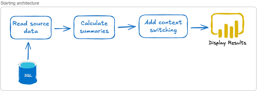
One approach is to just read the data directly from the SQL database. This would be the easiest solution. Once we read the data, we can perform our calculations, add in the context switching data, and display it:
This does raise a few interesting questions, though:
What happens if the source data changes in some way or if we can’t access the SQL database when we want to display our data?
How, exactly, are we going to store the results of the calculations and annotations?
Does this mean that every time we display the results we have to run through the entire pipeline, reading the data, performing calculations and then displaying our findings?
How does constantly accessing an external database impact our performance?
Data integrity and availability
We want our application to be highly available and reliable.
The problem is, we’ve created a dependency on an external system — the SQL database. If the external system changes or just isn’t available when we need it, we’ve got a problem. It would break our data pipeline. We need a solution that ensures both the integrity of the data as well as its availability.
The simplest solution is to just copy the data and keep a local cache of it. Whenever the source data is updated, we can update our local cache. If something goes wrong — for example, the data format changes or we can’t contact the SQL database — we can keep using our local cache until we fix the problem. That gives us high availability.
This also gives us a degree of certainty about the data format.
While the external SQL database might change, our internal cache can potentially remain constant. For example, let’s say the external database is using an Integer data type for activity duration, but at some point they decide to change it and start using a Time type instead. Since our local cache is under our own control, we have a few options:
Update our local cache to use
Timeas well, and change our pipeline code accordingly.Convert the incoming data from
Timeto anIntegerand store that. Leave our code as-is.Decide to use a completely different type, like
Duration, in our internal cache and make similar changes to our code.
Our strategy would depend on the situation — but we have options. We’ll examine a few different ones in a bit, but for now we’ll just note the internal cache in our architecture.
Adding a cache to the architecture might look something like this:
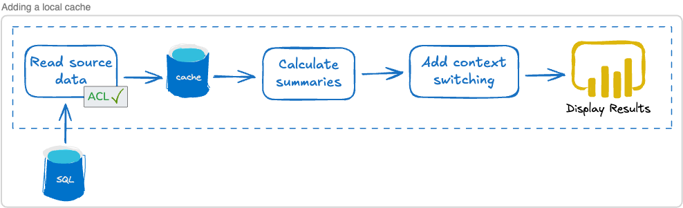
I’ve added an “ACL,” or “Anti-Corruption Layer,” to the intake process. ACLs are used to protect the data integrity of our domain — in other words, we don’t control the external SQL database but we do control our internal cache. That cache can, for instance, use a Duration to represent the passage of time regardless of how the SQL database represents time. The ACL is where we translate from the external format to our internal, domain-specific format.
It gives us a nice layer of isolation from external change. Generally speaking, creating isolation between services is a great strategy for improving reliability (as well as scalability — more on that later).
Benefits of isolation
I pointed out that by copying external data into our own system we are creating isolation. This is an important architecture topic for a few reasons:
Isolation means we are not inexorably dependent on an external system. If that external SQL database goes down, or the data changes, we can still function.
We also get architectural independence. If we decide to change the structure of our internal data cache, we can. It’s under our own control.
Being in control of our own data architecture also means we’re in control of our scalability. If our data analysis product becomes the hottest thing since sliced bread, we can scale up. We might add more servers to our cache, or we might evolve our architecture toward CQRS patterns — we’re in control, and it’s all hidden behind our product API.
From this perspective, copying data is a good idea. We need to remember there’s an external source of truth. But we remain in control of when we run data intake, how we change the data on the way in, and how our own data is structured.
Powerful, non-destructive annotation
Our original requirements include making sure that we maintain our source data integrity. The best possible approach in that regard requires two things.
First, we have to capture every record, in its entirety. That ensures we won’t miss anything important (including the possibility that something becomes important later, even though we thought it wasn’t important at first).
Second, we can’t change what we capture — we can only add to it. This means our analysis and data annotation can’t alter the source data — it’s immutable. We have to find a way to piggy-back or pair our new data with the raw source data.
We’ll leverage that in our code. Let’s say, for instance, you wanted to find out how many seconds of “out of sprint” work each user tracked in a sprint and you also want to make sure paid time off is not included in that number. Here’s a very simple example, using a snippet of Explorer code:
data
|> DF.group_by([“user_id”])
|> DF.filter(stereotype_code != "pto")
|> DF.summarise(out_of_seconds_sum: sum(out_of_sprint_seconds))
Data is just an array of raw data records. The group_by line groups all records with their respective team member. Then, with filter we make sure paid time off is not being included. And finally, we sum up all the out_of_sprint_seconds and put the result in a new variable, out_of_seconds_sum.
Two important things to note here: first, we haven’t altered the source data in any way. Second, we’ve annotated our data set by associating that new variable, out_of_sprint_sum, with our DataFrame.
We’ll explore this in depth soon. For now, I just wanted to give a quick taste of what we can do and explain why it’s valuable.
Tackling data analysis
We’ve decided how we’ll get the data, but there’s more work to do. How are we going to perform our calculations and store the results?
